EEG preprocessing, stage by stage · Blog

Walking through the seven preprocessing stages that take a raw LEMON recording from disk to the input my Conv-VaDE actually sees.

I get asked the same thing a lot: what exactly happens between “raw EEG file on disk” and “the 40x40 topomap the model trains on”. So this post walks through it on one participant (010004, eyes-closed), one fixed 76 ms window, every stage shown side by side. The point is that each stage does something specific and the figure shows you what.

The whole thing reuses one window. Same start time, same number of frames, same frame spacing. Anything that looks different between stages is the stage’s doing.

Setup

!pip install mne pycrostates

import numpy as np
import matplotlib.pyplot as plt
import mne
from mne.io import read_raw_eeglab
from pycrostates.datasets import lemon
from pycrostates.preprocessing import extract_gfp_peaks
from scipy.interpolate import griddata
import math as m

mne.set_log_level("WARNING")

plt.rcParams.update({
    "figure.dpi": 110,
    "image.cmap": "RdBu_r",
})

SUBJECT_ID = "010004"
CONDITION  = "EC"

L_FREQ     = 2.0
H_FREQ     = 20.0
CLIP_STD   = 5.0
TOPO_GRID  = 40

# One fixed window reused across every stage so figures are directly comparable.
START_SEC  = 30.0
N_FRAMES   = 20
STEP       = 1
N_COLS     = 10

Stage 0: raw from disk

Read the participant’s eyes-closed recording. No reference, no filter, nothing.

raw_fname = lemon.data_path(subject_id=SUBJECT_ID, condition=CONDITION)
raw_orig  = read_raw_eeglab(raw_fname, preload=True, verbose=False)
sfreq     = raw_orig.info["sfreq"]

s0 = int(START_SEC * sfreq)
window = raw_orig.get_data()[:, s0:s0 + N_FRAMES * STEP] * 1e6  # µV
t_ms = np.arange(window.shape[1]) / sfreq * 1000

fig, ax = plt.subplots(figsize=(12, 4))
ax.plot(t_ms, window.T, color="gray", alpha=0.4, linewidth=0.5)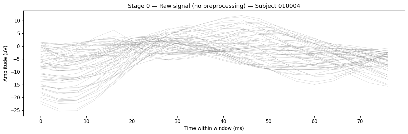

Stage 0: raw signal, all channels, 76 ms window

Each gray line is one channel. The mean drifts because there’s no reference applied yet, and the slow envelope is unfiltered low-frequency drift.

Stage 1: pick EEG channels

Drop anything that isn’t an EEG channel. EOG, ECG, status channels are gone after this. No figure: it’s a channel-set change, not a signal change.

raw_picked = raw_orig.copy().pick("eeg")

Stage 2: average reference

Re-reference to the mean across all kept EEG channels. After this, the mean across channels at any instant is approximately zero. That’s the property the next stages assume.

raw_ref = raw_picked.copy().set_eeg_reference("average", verbose=False)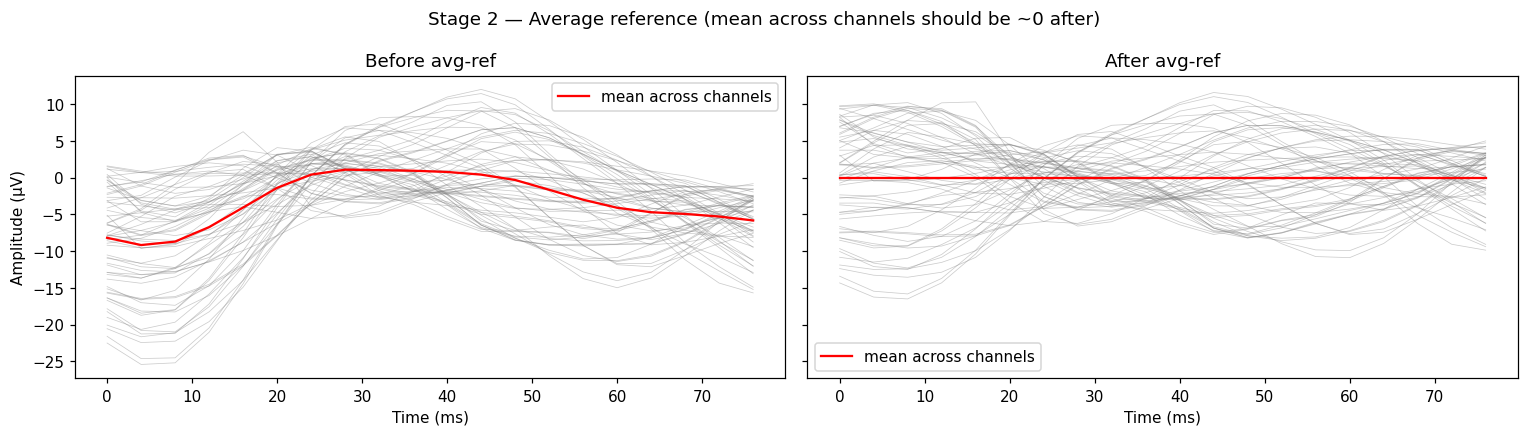

Stage 2: butterfly plot before and after average reference. Mean across channels in red.

Left panel: the red line (mean across channels) sits well below zero, drifting with the recording. Right panel: red sits on zero across the window. That’s what “average reference” means in one picture.

Stage 3: bandpass 2-20 Hz

FIR filter, zero-phase. The passband covers the resting-state bands of interest for microstate analysis: roughly the upper end of delta, theta, alpha, and the lower beta. Anything below 2 Hz is slow drift; anything above 20 Hz is muscle and line noise.

raw_filt = raw_ref.copy().filter(l_freq=L_FREQ, h_freq=H_FREQ,
                                  method="fir", phase="zero", verbose=False)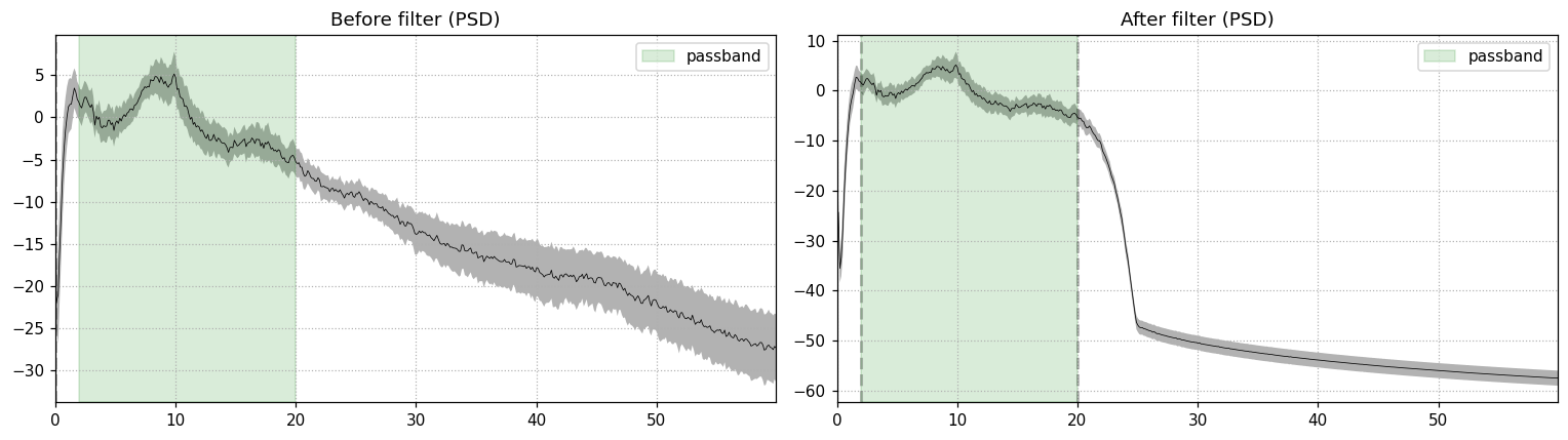

Stage 3: power spectrum before and after the bandpass, with the passband shaded

The right panel shows the floor dropping by 40+ dB above 20 Hz. The passband (green shading) is preserved. The alpha bump near 10 Hz is intact, which is what you want for an eyes-closed recording.

Stage 4: sequential topomaps

Now I sample 20 consecutive frames from the filtered signal, 4 ms apart at 250 Hz. Each frame becomes a topomap (interpolated scalp potential). Because the frames ARE consecutive in time, you should see the field evolve smoothly from one to the next.

data_filt = raw_filt.get_data()
sample_idx = np.arange(s0, s0 + N_FRAMES * STEP, STEP)
frames = data_filt[:, sample_idx]
times_ms_abs = sample_idx / sfreq * 1000

vmax = np.max(np.abs(frames))
vmin = -vmax

n_rows = int(np.ceil(N_FRAMES / N_COLS))
fig, axes = plt.subplots(n_rows, N_COLS, figsize=(2.0 * N_COLS, 2.4 * n_rows))
axes = np.atleast_1d(axes).flatten()
for i in range(N_FRAMES):
    mne.viz.plot_topomap(frames[:, i], raw_filt.info, axes=axes[i],
                          show=False, cmap="RdBu_r", vlim=(vmin, vmax),
                          sensors=False, contours=6, outlines="head")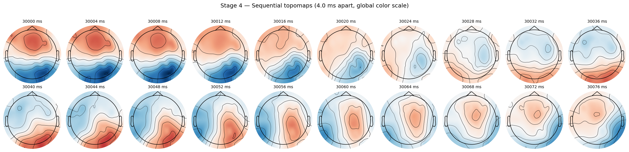

Stage 4: 20 sequential topomaps, 4 ms apart, global color scale

Top row: the anterior red blob slowly fades and shifts. Bottom row: a posterior red blob emerges and intensifies. That smoothness is the signature of consecutive-time sampling.

Jagged frame-to-frame transitions on a sequential plot like this would mean something upstream is wrong (wrong sampling rate, dropped samples, polarity flip applied where it shouldn’t be). I use this exact view as a fast smoke test when I touch the preprocessing code.

Stage 5: geometry check (custom griddata 40x40)

The model trains on 40x40 images, not on the channel vector directly. I project the 3D electrode positions to 2D and interpolate the channel values onto a 40x40 grid with cubic griddata. Three sanity panels: (a) the projected electrode positions look symmetric, (b) the custom griddata output matches what (c) MNE’s reference plot_topomap produces for the same sample.

def cart2sph(x, y, z):
    r = m.sqrt(x*x + y*y + z*z)
    elev = m.atan2(z, m.sqrt(x*x + y*y))
    az = m.atan2(y, x)
    return r, elev, az

def azim_proj(pos):
    _, elev, az = cart2sph(*pos)
    rho = m.pi / 2 - elev
    return rho * m.cos(az), rho * m.sin(az)

locs_3d = np.array([ch["loc"][:3] for ch in raw_filt.info["chs"]]) * 1000
pos_2d = np.array([azim_proj(p) for p in locs_3d])

def make_topo(vals):
    # First mgrid dim varies y (anterior-posterior), second varies x (left-right).
    # Previously these were reversed, which rotated topomaps 90 degrees off
    # standard EEG convention. This is the rotation fix.
    gy, gx = np.mgrid[
        pos_2d[:, 1].min():pos_2d[:, 1].max():TOPO_GRID*1j,
        pos_2d[:, 0].min():pos_2d[:, 0].max():TOPO_GRID*1j,
    ]
    return griddata(pos_2d, vals, (gx, gy), method="cubic", fill_value=0)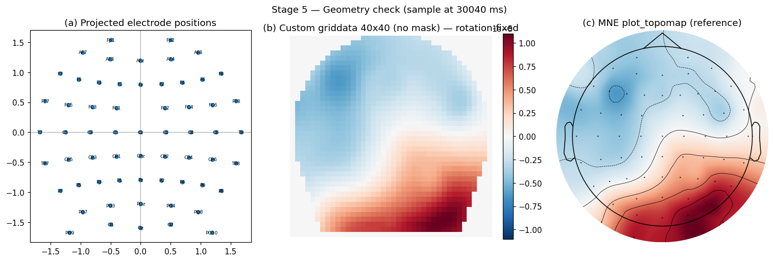

Stage 5: electrode positions, custom griddata 40x40, MNE plot_topomap reference for the same sample

The corners of the 40x40 image are fill_value=0 from griddata. Those four corners are not brain signal. Every loss and per-pixel metric in my training code masks them out (see mask_utils.py in the repo). I’ll write a separate post on that masking convention.

Stage 6: z-score normalisation, clip at ±5

Compute the mean and std over the full filtered recording (proxy for the train split during the actual training pipeline). Subtract, divide, clip extremes. The model sees the result.

all_data = raw_filt.get_data()
mu = float(all_data.mean())
sd = float(all_data.std()) or 1e-12
frames_z = np.clip((frames - mu) / sd, -CLIP_STD, CLIP_STD)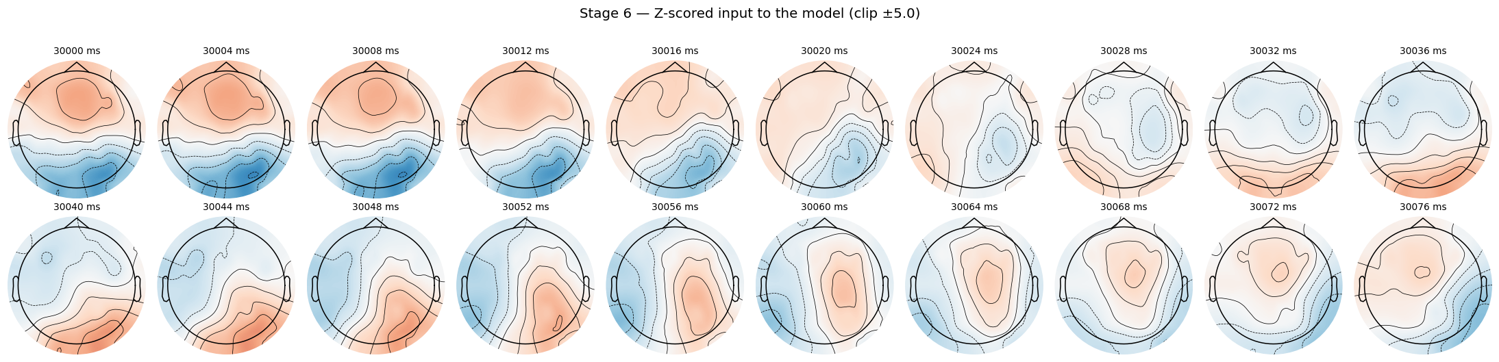

Stage 6: the same 20 frames as Stage 4 but in z units, clipped at ±5

Same window, same evolution as Stage 4, but the color scale is now z-units. This is the exact input the model trains on, modulo polarity-flip augmentation that happens at the dataset level (separate post coming on polarity).

Stage 7: GFP peaks (and why they don’t look like Stage 4)

Stage 4 was 20 consecutive samples. Stage 7 is 20 consecutive GFP peaks. Those are not the same thing. Adjacent GFP peaks can be 50 to 200 ms apart, and polarity at each peak is arbitrary (peaks are detected on instantaneous global field power, which is the absolute spatial standard deviation).

peaks = extract_gfp_peaks(raw_filt, min_peak_distance=3,
                          reject_by_annotation=True)
peaks_data = peaks.get_data()
n_peaks = peaks_data.shape[1]
duration_s = raw_filt.n_times / sfreq

PEAK_START = 1059
peak_range = np.arange(PEAK_START, PEAK_START + N_FRAMES)
peak_range = peak_range[peak_range < n_peaks]
peak_frames = peaks_data[:, peak_range]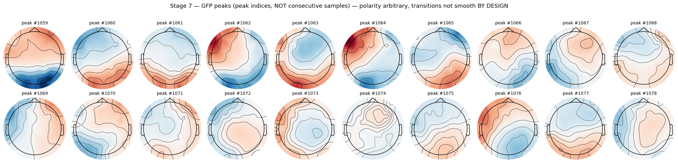

Stage 7: 20 consecutive GFP peaks (peak indices, not consecutive samples), polarity arbitrary

Compare this grid against Stage 4. Same plotting code, same layout, but the frame-to-frame relationship is gone. Each cell is a distinct topographic configuration captured at a moment of locally-maximal global field power. The titles are peak indices, not millisecond timestamps.

Non-smoothness between consecutive peaks is by design. Microstates are stable topographic configurations separated by rapid reorganisation events. The reorganisation is what GFP peak detection captures. Plotting consecutive peaks and expecting them to evolve smoothly like the Stage 4 frames is a category error.

This is also why polarity invariance matters. If peak #1059 happens to be polarity-flipped relative to peak #1060, they may represent the same underlying configuration. The clustering pipeline (and my model) has to be invariant to that sign. More on that in the next post.

Why this matters

Each stage encodes a methodological choice. Get the wrong reference, or the wrong bandpass, or skip the corner mask after griddata, and your microstate alphabet is measuring artefacts instead of brain configurations. Going stage by stage on a fixed window means I can verify each step visually instead of trusting the code.

Code lives in microstate-architecture-search, the public companion to the XAI 2026 paper.

Next post: the topomap masking convention, and why every metric in the project ignores the four corners of the 40x40 image.