Pick a K. Train the model. Now score it.
If you only report one number, you’ve made two choices the reader can’t see. Which metric did you use, and which representation space did you compute it in. Both choices change the answer. The four-quadrant framework spells out both axes so the verdict on “is this a good model” stops being a function of which number happened to look best.
The 2x2 grid
| Quadrant | Space | Distance | What it answers |
|---|---|---|---|
| Q1 | Latent 32D | Euclidean (sklearn) | How well the encoder separates clusters in its own learned coordinates |
| Q2 | Latent 32D | ∣1/corr∣-1 (pycrostates) | Same space, but with the correlation distance EEG people are used to |
| Q3 | Topomap 1600D | Euclidean | How well the decoded reconstructions separate, pixel by pixel |
| Q4 | Topomap 1600D | ∣1/corr∣-1 | The closest direct comparison to the classical ModKMeans baseline |
Inside each quadrant the project reports four scores: silhouette, Davies-Bouldin, Calinski-Harabasz, Dunn. That’s 16 numbers per trained model. Sounds excessive until you watch them disagree.
Metrics disagree, even inside one quadrant
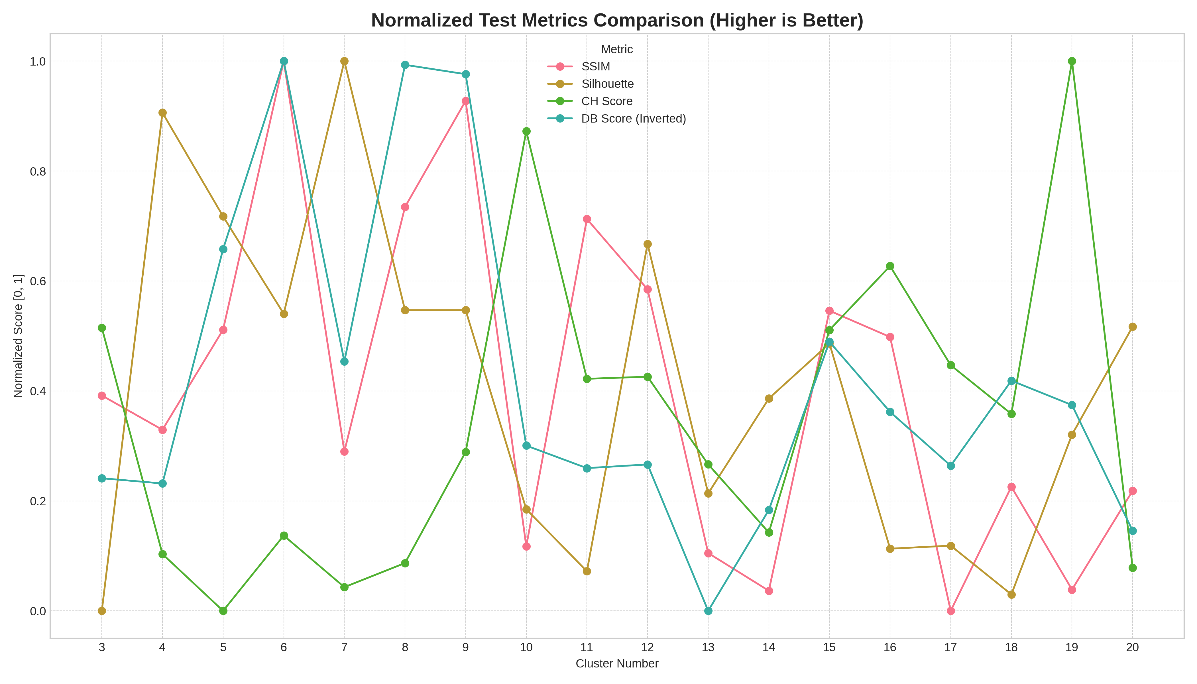
Test-split scores from one participant. Each metric normalised to [0,1] so the lines are comparable. Look at where each one peaks: Silhouette and DB-inverted both like K=6, but SSIM tops out around K=8-9, and Calinski-Harabasz keeps climbing until K=19. Pick whichever one feels most authoritative and you’ve picked a different best-K.
That’s already a problem with a single quadrant. Pick “the score” and you’ve picked a story. There’s no global ranking on which metric is right, because each measures a slightly different shape of cluster quality (compactness, separation, density, total within-cluster scatter).
The same metric, four quadrants, four answers
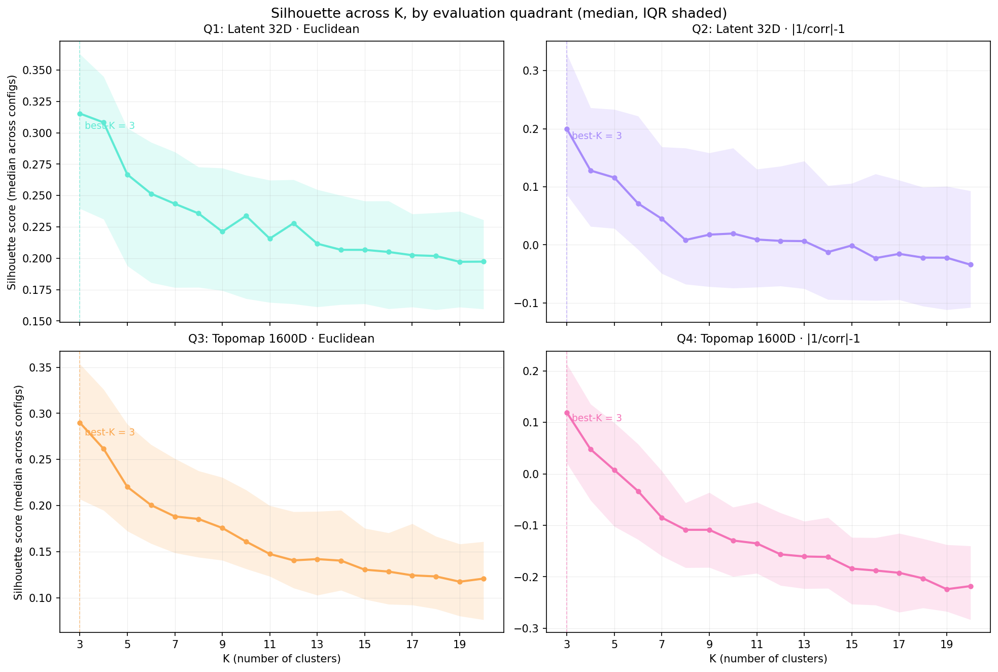
4,832 models from the sweep, aggregated by K. Best-K agrees across all four quadrants on silhouette (K=3 every time, marked with a dashed line). But the magnitudes are very different. Q1 peaks at 0.315 in the latent space the encoder optimised; Q4, the ModKMeans-comparable view, peaks at 0.119. Same model, half the silhouette score, because the evaluation lens is harder.
Two things to take from this chart.
Magnitudes carry information about the space, not just the model. Q1 looks great because the encoder is doing what it’s supposed to do: pulling clusters apart in its own latent coordinates. Q4 looks worse because once you decode back to topomap space and use the correlation distance EEG people care about, the separation gets noisier. Reporting only Q1 would let you publish a model that looks crisp in latent space but doesn’t actually compete with the classical baseline.
The IQR width tells you how brittle the configuration choices are. Wide bands at low K mean the silhouette score is sensitive to depth/ndf/latent-dim choices at those K. Narrow bands at high K mean configurations have converged to similar (lower) scores. That’s design-space information you’d never see from a single best-config number.
SSIM is not a cluster-validity score in disguise
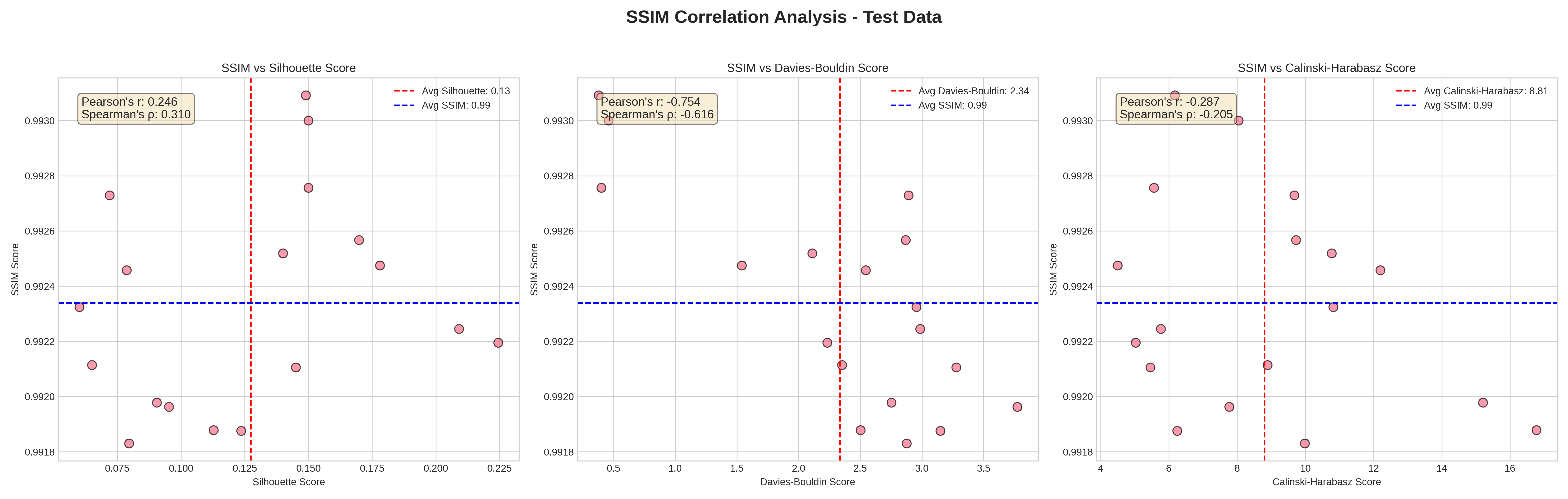
SSIM (reconstruction fidelity, x-axis runs vertical here) plotted against each cluster-validity score on the test split. SSIM barely moves (everything sits between 0.991 and 0.993), but Silhouette ranges 0.05 to 0.225 across the same models, Davies-Bouldin ranges 0.5 to 4.0, CH ranges 5 to 16. The model can reconstruct well and cluster badly, or reconstruct well and cluster well. Reconstruction is not a substitute.
This matters because reconstruction loss is what the VAE actually optimises. A reasonable instinct is “if recon loss is low, the model is good”. The chart says no: SSIM stays near-perfect across the entire sweep while cluster quality varies by 4-5x. You have to evaluate clustering directly.
Why Q4 anchors the comparison to ModKMeans
Classical EEG microstate analysis runs modified k-means in electrode space using the |1/correlation|-1 distance. That’s exactly Q4: topomap 1600D, correlation distance. So Q4 is the only quadrant where “my VaDE model” and “the canonical ModKMeans baseline” speak the same language and the same metric without translation. Q1 and Q2 are encoder-private numbers. Q3 is what an image-pixel statistician would compute. Q4 is what an EEG clinician would.
If you only have time to look at one quadrant, look at Q4. If you have time for two, add Q1, because that’s where the encoder lives. The other two are useful for diagnostic work, not for headline claims.
The point
Every score the project reports lives somewhere on the (metric, quadrant) grid. Don’t quote one and call it the answer. Quote the position on the grid alongside the number. “Q4 silhouette = 0.12 at K = 4” tells the reader more than “silhouette = 0.12”, because the next person can compare against ModKMeans or against a paper that worked in latent space without inventing a translation.
Next post: polarity invariance. Why two topomaps that are sign-flipped versions of each other should not be measured as different states, and how the project enforces that through sign-flip data augmentation and an invariance loss on the encoder.